Projects

N3D - Integration of the Navier-Stokes equations in
3 dimensions for direct numerical simulations

N3D is a solver for highly accurate computation of transitional and turbulent flows, developed at the Institut für Aerodynamik und Gasdynamik (IAG), Stuttgart of University. It is based on the vorticity-velocity formulation of the Navier-Stokes equations for an incompressible fluid.

The code is optimized for highest processing speed on each single vector-type CPU. To obtain optimal performance on multinode vector supercomputers, N3D applies a hybrid approach employing two fundamentally different parallelization techniques at the same time: a directive-based shared-memory OpenMP parallelization is combined within one node with an explicitly coded distributed-memory MPI parallelization.

The performance on vector supercomputers can be about 50-60% of the theoretical peak performance. The code scales very well in distributed-/shared-memory environments with a high memory bandwidth such as the NEC SX series.

Features:

• High-order discretization in space (compact finite differences of 4th/6th order in streamwise and wall-normal direction, complex spectral Fourier ansatz in spanwise direction) and time (4th order Runge-Kutta).
• Reduction of aliasing errors by alternating up- and downwind-biased finite differences in time for streamwise derivatives (high-order McCormack-type scheme), while at the same time keeping the favorable dispersion characteristics of a central scheme.
• Pseudo-spectral computation of the non-linear terms in physical space by means of Fast Fourier Transforms.
• Multi-grid technique for the computation of a Poisson equation for the wall-normal velocity to accelerate convergence or direct method based on a Fourier expansion.
• Non-reflective buffer domain at the outflow boundary.
• Total-flow and disturbance formulation - the latter requires the knowledge of a corresponding laminar flow solution.
• Cartesian grids with the possibility of near-wall refinement in wall-normal direction by means of wall-zones or grid-stretching.
• Large-Eddy Simulation mode by adding a turbulence model similar to the approximate deconvolution method.

Applications:

• Fundamental research in fluid dynamics: emphasis on complex, highly unsteady flow physics.
• Studies of transition in straight and swept-wing boundary layers with arbitrary pressure gradients, including separated flows, for Reynolds numbers relevant in engineering applications.
• Development and testing of passive and active flow-control strategies, like boundary-layer suction or upstream flow deformation to delay transition in swept-wing boundary-layers or unsteady forcing to remove separation regions.

The N3D application was reworked in several stages to provide better scalability and better single CPU performance. The improvements are to enable better utilization of a large machine. Traditionally the program have been run on one maybe two SX node. The hight performance of the old machines in comparison to their contemporary compeditors made the SX platform the platform of choise for its high performance. As a single CPU system or even an SMP machine have reached the limits of what is possible in performance the direction is to run constellations of fast machines. This introduce new problems as domain decomposition.

Scaling becomes very important and even if a problem is dividable most problems are not easilly parallelized. As the machine is very large with 72 nodes, one wants to take advantage of the power of these nodes to calculate larger more detailed cases. N3D scales with the dimensions of the dataset, this means that distributing the code on less powerful processors, increases the need for a larger domain, which in turn increases the need for computepower. The SX-8 nodes in themselfes already are very powerful and by simply scaling the problem from the old usage of one to two nodes, to ten nodes improves throughput and research abilites of the IAG.

Tunings

The N3D is relying on sine and cosinus transforms, since the Z dimension is represented in frequency space. These transforms were compiled from source. The sine transform uses sines only as a complete set of functions in the interval from 0 to 2p, and, the cosine transform uses cosines only. By contrast, the normal Fast Fourier Transforms (FFT) uses both sines and cosines, but only half as many of each. Sine and cosinus transform are not a part of the highly optimized mathematical libraires, however FFTs are. By combining sine and cosine transform data, it is possible to use the FFT to do the transform.

N3D does have a rather costly all-to-all communication, when dealing with the frequency domain Z direction of the dataset. One target was to overlap the communication, which can only be made by one CPU of the eight CPU node, with meaningfull work, increasing the throughput. Another step is to use the SX-8 global memory option in MPI communication.

The N3D have the data domain decomposed in the Z direction. As the FFT transform needs to be solved a redistribution of the data have to take place. The FFT needs to have access to all values in the Z direction. The way it is made is that a new simple domain decomposition is made over the X dimension. This allows for a MPI all-to-all distribution which at the end permtits one thread to work on a part of X but with the full Z dimention at its disposal. In the earlier version the communication dealt with the full dataset at once. By breaking down also the Y direction in independant blocks, it is possible to create a pipelined loop. Where the comminication of blocks with MPI can be overlapped with calculating the FFT and domaindecomposing data in other blocks. Thus effectivly overlapping the communication done by one CPU with FFT calcultion that is done with remaining CPUs.

Instead of doing MPI communication and FFT of the whole data, first MPI communication is done on a Y layer. As that is transported, the next layer is transported. The first layer can that already have been communicated can then be calculated on by the FFT algorithm and so on.

As the routines had been adapted for this division in Y, the step of changing the MPI communication was taken. A communciation pattern using MPI_Put was introduced. This gives each thread the possibility to exchange data to global buffers. This more asyncronous communication can also be achieved on other implementing the MPI_ALLOC_MEM call to allocate global memory.

Results

The tuningsteps brought different improvments, single cpu performance and scaling speedups.

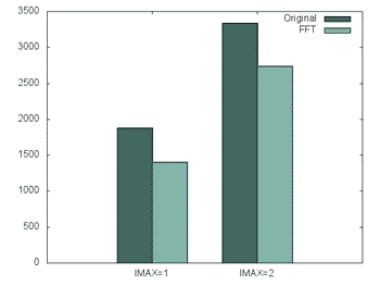
Figure 1. The performance improvements of changing the transforms

The initial change, moving from homemade sine and cosinus transforms gave a direct improvement of 34% for the IMAX=1 path and 22% for the IMAX=2 path. The larger improvement in the IMAX=1 path can be attributed to the symetricy in the frequency data that IMAX=1 denotes. Less data is used to reach the result, giving the IMAX=1 path an advantage over IMAX=2. Both versions are used in research depending on the problems investigated.

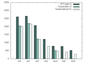
Figure 2. The performance improvements of the scaling tunings

In the scaling step most concentration was put into IMAX=2 that is the more complex setup. The results from the scaling work can be seen in the plot below. The Z dimention that was used in these tests were 119. Still there are some improvements in the single threaded part, due to the fact that in the work to scale the performance, there were also rewrites that limited the numbers of copies of arrays made. Also the tridiagonal solver was improved with some directives. The different numbers refering to I/O means writing restart files which is something that is done at the last cycle. As it became evident that it affected some measurements separate runs were made without this. The effect was limited, but measured.

Looking at the 4 cpu per MPI thread numbers, scaling was improved from 3.3 to 4.3 including I/O, going from 1 to 5 nodes. This with a theoretical limit of 5. For the smaller case as 119 using 8 CPU per thread limits the amount of data each CPU works with, thus making the vectors smaller etc. Still going from 5 nodes to 10 gives a scaling factor of 1.70 compared to 1.52 in the version without scaling tunings.

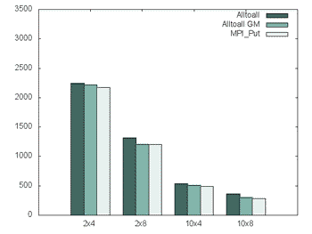
Figure 3. MPI - Global memory

In the work of improving the scaling there were also a change from using a normal MPI All-to-all to use the SX-8 global memory segment and to further improve the communication using an asyncronus scheme with MPI_Put and global memory. As can be seen just using global memory the time, and that is mostly due that internal buffer copying is reduced.

TeraFlop and production

The performance one teraflop of the program was reached with a Z dimension of 210. Using 70 nodes 1.15 teraflop was reached. Still higher performance can be reached with a larger case. The 210 number is a bit low to fully utilize the scaling effects of the vector computer, which actually works better when there are some substantial data to be calculated per node. Z = 119 was used for the tunings, but the Z = 210 was used to allow the higher number of nodes, due to the way the domain decomposition is done.

Still for this size of the problem that do reach one teraflop, it is very efficient in the range 5 - 15 nodes. This is an area which is more reasonable for production. As the research needs more detailed analysis, growing the problemsize will not be a problem.

Contact:

Markus Kloker / Ulrich Rist
Institut für Aerodynamik und Gasdynamik
Universität Stuttgart
Phone: +49 711 685-3427/-3432

Fredrik Svensson
Application Analyst
NEC HPCE - EHPCTC
Phone: ++49-711-78055-17